Finite Elements from Scratch
Background
"The finite element method (FEM), is a numerical method for solving problems of engineering and mathematical physics." -Wikipedia
One of the elementary formulations of fem in structural engineering is the truss. They are very basic, but have a lot of utility.

When one designs a truss, especially in the preliminary stages some assumptions are usually made to simplify the procedure. For instance, members are assumed to carry only tension or compression load. This means that we can only load the truss at the nodals points. Depending on how the connection is designed and detailed, these assumptions can be quite close to how the structure actually will behave in the real world.
So, what's so special about having a member with only axial loading? Well, there's a property of the material itself we can take advantage of. Most materials have a property of 'linear elasticity' when the material is stretched or compressed a very small amount. A material like steel is quite ductile, and so this range of linear elasticiticy is quite large, as compared to something like ceramics. This means if we push or pull on some steel with a small force, it will displace a proportional amount. If we double our applied force, its displacement will double as well. Also if we release our force, the material will go back to its original configuration. So as long as we deform the material elastically, we won't waste any energy deforming it plastically.
If you have ever taken a physics class, you may know that a spring has these exact same properties. Therefore, we can idealize all the members in our truss as just simple springs.
Building up to direct stiffness method
A zero dimensional spring equation looks like this.
$$
K \cdot u = F
$$
This relates the force required to any deformation of the spring. The force and deformation are linearly proportional by \$K\$, the spring constant. The constant \$K\$ has units of [force/distance] e.g. [pounds/in] or [kilograms/meter]. For example, if \$K = 50 lb/in\$, it would take \$50lb\$ of force to displace the spring \$1\$ inch, and \$100lb\$ to displace the spring \$2\$ inches. The stiffness in our truss members is similar:
$$
K = \frac{EA}{L}
$$
\$E\$ is Young's Modulus, \$A\$ is the cross sectional area, and \$L\$ is the length of the bar. The only scary thing here is probably \$E\$, but it's not too crazy. It's kind of like stiffness, but it's normalized. Instead of [force/distance] we have [stress/strain]. Stress is like the normalized force, it's the amount of force over the area of the element. Strain is like the normalized displacement, it's calculated by (change in length/original length) or percent elongation.
Let's develop this a bit more and put it in matrix form. This will allow us to relate the force on one side of the bar to force on the other.
$$
\frac{EA}{L}
\left[\begin{array}{cc}
1 & -1\\
-1 & 1 \\
\end{array}\right] \cdot
\left[\begin{array}{c}
u_1 \\
u_2 \\
\end{array}\right] =
\left[\begin{array}{c}
f_1 \\
f_2 \\
\end{array}\right]
$$
Now we have our one dimensional spring equation. Instead of a single displacement, we have a displacement vector. We can displace both sides of the spring independently and find what the resultant forces on each side will be.
Examples:
Displace the right node 1 unit to the right
$$
\frac{EA}{L}
\left[\begin{array}{cc}
1 & -1\\
-1 & 1 \\
\end{array}\right] \cdot
\left[\begin{array}{c}
0 \\
1 \\
\end{array}\right] =
\left[\begin{array}{c}
f_1 \\
f_2 \\
\end{array}\right]\\
f_1 = \frac{-E A}{L}, f_2 = \frac{E A}{L}
$$
This makes sense, because if we displace the right side by a unit, we need a force in the equal and opposite direction on the left side to not drag that side along.
Displace both nodes \$1\$ unit to the right
$$
\frac{EA}{L}
\left[\begin{array}{cc}
1 & -1\\
-1 & 1 \\
\end{array}\right] \cdot
\left[\begin{array}{c}
1 \\
1 \\
\end{array}\right] =
\left[\begin{array}{c}
f_1 \\
f_2 \\
\end{array}\right]\\
f_1 = 0, f_2 = 0
$$
This makes sense, because if we displace both sides at the same time, the distance between them does not change. It would be as if we just translated the spring across the table and did not strech it. We don't need some force holding it in a deformed configuration.
That's cool, but one dimensional structures are lame. I want a two dimensional structure to build a bridge! Well, it's not that much more difficult. We just need to add a \$y\$ degree of freedom (dof) on each side of the spring. We can also couple our \$x\$ and \$y\$ dofs into one angle from the \$+x\$ direction to simplify our matrix. And so with some magic (rotational matrix) we can get the following:
Step 1 - Local Stiffnes Matrix

This is our local stiffness matrix, also known as \$K^e\$. It has all the same properties as our one dimensional stiffness matrix, but it takes into account \$(x,y)\$ displacements at each side of the spring. This gives us a total of four degrees of freedom.
You may begin to see how powerfull this method can be. We can now iterate through all of our elements and just calculate the angle and length from its nodes. This will give us \$i\$ local stiffness matrices, where \$i\$ is the number of elements. For example if we have \$3\$ elements in our truss, we can calculate our \$3\$ local matrices for each element.
Let's go through an example.

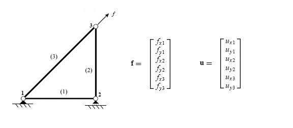
If we calcualted the local stiffness matrices for the figure above (\$EA = 1\$, \$L(1,2)=1\$), you would find:
$$
\hspace{50pt}\begin{array}{cccc}1 & 2 & 3 & 4\\\end{array} \\
K(1) =
\begin{array}{c}
1 \\
2 \\
3 \\
4 \\
\end{array}
\left[\begin{array}{cccc}
1 & 0 & -1 & 0\\
0 & 0 & 0 & 0\\
-1 & 0 & 1 & 0\\
0 & 0 & 0 & 0\\
\end{array}\right]
$$
$$
\hspace{50pt}\begin{array}{cccc}3 & 4 & 5 & 6\\\end{array} \\
K(2) =
\begin{array}{c}
3 \\
4 \\
5 \\
6 \\
\end{array}
\left[\begin{array}{cccc}
0 & 0 & 0 & 0\\
0 & 1 & 0 & -1\\
0 & 0 & 0 & 0\\
0 & -1 & 0 & 1\\
\end{array}\right]
$$
$$
\hspace{50pt}\begin{array}{cccc}1 & 2 & 5 & 6\\\end{array} \\
K(3) =
\begin{array}{c}
1 \\
2 \\
5 \\
6 \\
\end{array}
\left[\begin{array}{cccc}
0.64 & 0.48 & -0.64 & -0.48\\
0.48 & 0.36 & -0.48 & -0.36\\
-0.64 & -0.48 & 0.64 & 0.48\\
-0.48 & -0.36 & 0.48 & 0.36\\
\end{array}\right]
$$
Where the numbers outside the array correspond to the global matrix indicies.
Step 2 - Assemble local matrices into the global matrix
These local matricies are uncoupled, and so they don't really tell us much about the global system of the truss, or how to solve for the displacements with given forces. However, we can do something called matrix assembly to put them all into one big global stiffness matrix. This will couple all of our local element equations so we can solve our system of equations.
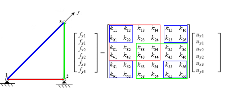
We do this by matching the local degrees of freedom to our global degrees of freedom, then add our local to our global matrix.
Since our global truss has 3 nodes and each node has \$2\$ dofs \$(x,y)\$, our global matricies are of size 6. \$K \in \mathbb R^{6 \times 6}, F \in \mathbb R^{6 \times 1}, u \in \mathbb R^{6 \times 1}\$. If we layed out the dof number for each row/column of our stiffness matrix we would get the following:
$$
\hspace{35pt}\begin{array}{cccccc}1 & 2 & 3 & 4 & 5 & 6\\\end{array} \\
K =
\begin{array}{c}
1 \\
2 \\
3 \\
4 \\
5 \\
6 \\
\end{array}
\left[\begin{array}{cccccc}
0 & 0 & 0 & 0 & 0 & 0\\
0 & 0 & 0 & 0 & 0 & 0\\
0 & 0 & 0 & 0 & 0 & 0\\
0 & 0 & 0 & 0 & 0 & 0\\
0 & 0 & 0 & 0 & 0 & 0\\
0 & 0 & 0 & 0 & 0 & 0\\
\end{array}\right]
$$
From step 1, the global dofs of \$k(1)\$ were \$1,2,3,4\$. This means we just add them index by index into our global stiffness matrix.
$$
\hspace{35pt}\begin{array}{cccc}1 & 2 & 3 & 4\\\end{array} \\
k(1) =
\begin{array}{c}
1 \\
2 \\
3 \\
4 \\
\end{array}
\left[\begin{array}{cccc}
k_{11} & k_{12} & k_{13} & k_{14}\\
k_{21} & k_{22} & k_{23} & k_{24}\\
k_{31} & k_{32} & k_{33} & k_{34}\\
k_{41} & k_{42} & k_{43} & k_{44}\\
\end{array}\right]
$$
If we match up the indicies, we can just add:
$$
K_{11} += k_{11}\\
K_{12} += k_{12}\\
K_{13} += k_{13}\\
K_{14} += k_{14}\\
K_{21} += k_{21}\\
...
$$

We can see if we do this for all three elements, we can match up where they will go in the global matrix with colors. This is shown in the figure below.

Step 3 - Add bounds on the stiffness matrix, and modify the force vector

We are almost done! But there is one final important step. If we were given an arbitrary force vector and tried to find the displacements, our truss would just fly away to infinity. This is because there are no boundary conditions! There is nothing yet holding on to it, resisting the forces. But guess what? There's another neat trick we can use. This will keep everything in matrix form and give us the answers we want when we solve our system of equations.
All we do is remove the influence of the node on the force vector. For this example, we will assume the constraint on dof1 is set to \$g\$.
For the general case, we just set \$dof1 = g\$ in the force vector, and subtract g* the column of \$K\$ with dof1 = 0. If \$g=0\$, we just need to set \$dof1 = 0\$ in the force vector.
$$
F =
\left[\begin{array}{c}
F_1\\
F_2\\
F_3\\
\vdots\\
F_n\\
\end{array}\right] \Rightarrow
\left[\begin{array}{c}
g\\
F_2\\
F_3\\
\vdots\\
F_n\\
\end{array}\right] - g
\left[\begin{array}{c}
0\\
K_{21}\\
K_{31}\\
\vdots\\
K_{n1}\\
\end{array}\right]
$$
Then we just restrain our stiffness matrix. This can be done by zeroing out the row and column of \$dof1\$, then setting \$(dof1,dof1)=1\$ as shown below.
$$
K =
\left[\begin{array}{cccc}
K_{11} & K_{12} & \cdots & K_{1n}\\
K_{21} & K_{22} & \cdots & K_{2n}\\
\vdots & \vdots & \ddots & \vdots\\
K_{n1} & K_{n2} & \cdots & K_{nn}\\
\end{array}\right] \Rightarrow
\left[\begin{array}{cccc}
1 & 0 & \cdots & 0\\
0 & K_{22} & \cdots & K_{2n}\\
\vdots & \vdots & \ddots & \vdots\\
0 & K_{n2} & \cdots & K_{nn}\\
\end{array}\right]
$$
Step 4 - Solve with linear algebra
Now we are finally back to our equation of a spring. However, in this case each variable below is an array or vector of size \$n\$, where \$n\$ is the number of \$nodes \times 2\$.
$$
\mathbf{K} \cdot \mathbf{u} = \mathbf{F}
$$
We can simply solve this system of equations by taking the inverse of the stiffness matrix. This gives us:
$$
\mathbf{u} = \mathbf{K}^{-1} \cdot \mathbf{F}
$$
This can be easily solved by a computer. For example Python:
u = np.linalg.solve(K, F)
Rules
- Input data type can for the most part be changed for your needs. However, it should be human-readable, or at least reasonable to be able to change the input for a new structure easily.
Example input
E = .
A = .
nodes = [., ., ...]
elements = [., ., ...]
forces = [., ., ...]
bounds = [., ., ...]
Example output
[., ., ...]
- Output can be in any form, as long as it's in order of dof.
- Inbuilt FEM functions not allowed. You must construct and assemble your matrices yourself. Inbuilt linear algebra is fine.
Test Cases
From UNM example in references:
E = 29500
A = 1
nodes = [[0,0],[40,0],[40,30],[0,30]]
elements = [[1,2],[2,3],[1,3],[3,4]]
forces = [[0,0],[20,0],[0,-25],[0,0]]
bounds = [[0,0],[None,0],[None,None],[0,0]]
Output:
[0.0 0.0 0.027 0.0 0.006 -0.022 0.0 0.0]
Large Truss Input:
E = 29000
A = 25
nodes = [[0,0],[100,0],[200,0],[300,0],[0,100],[100,100],[200,100],[300,100],[400,100]]
elements = [[1,2],[1,5],[1,6],[2,3],[2,6],[2,7],[3,4],[3,7],[3,8],[4,8],[4,9],[5,6],[6,7],[7,8],[8,9]]
forces = [[0,-10],[0,-10],[0,-10],[0,-10],[0,0],[0,0],[0,0],[0,0],[0,-10]]
bounds = [[0,0],[None,None],[None,None],[None,None],[-0.01,0],[None,None],[None,None],[None,None],[None,None]]
Output:
[ 0. 0. -0.008 -0.025 -0.012 -0.061 -0.014 -0.1 -0.01 0. 0.004 -0.019 0.012 -0.057 0.016 -0.098 0.018 -0.136]
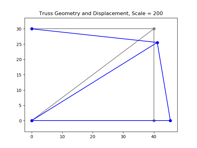
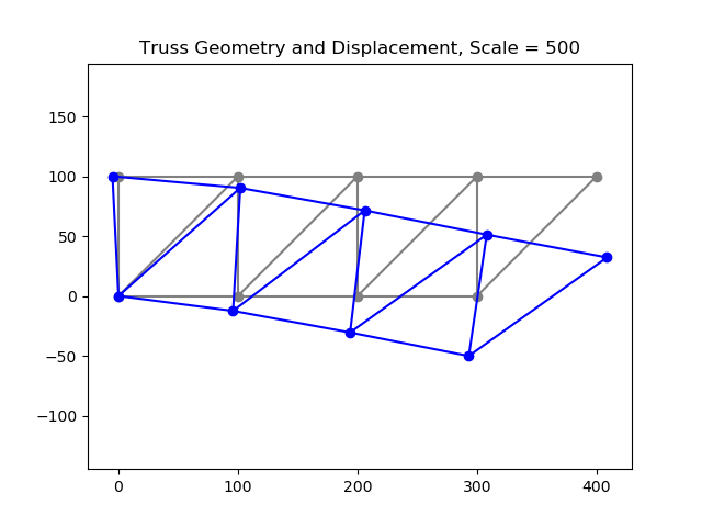
Here is what the geometry and displacement looks like for the test cases so you can visualize it.


References
Here are some references that may be useful if you are looking for some more in-depth information.
http://www.unm.edu/~bgreen/ME360/Finite%20Element%20Truss.pdf
https://engineering.purdue.edu/~aprakas/CE474/CE474-Ch5-StiffnessMethod.pdf
http://people.duke.edu/~hpgavin/cee421/truss-method.pdf
http://ocw.ump.edu.my/pluginfile.php/9806/mod_resource/content/2/7_Plane_Truss_Example.pdf
https://nptel.ac.in/content/storage2/courses/105105109/pdf/m4l24.pdf
And lastly, here is some working python 3 code that I wrote. It should lay out all the steps cleanly.
import numpy as np
from math import sqrt,sin,cos,acos

def ex_unm():
    """Example - Verification from UNM"""
    print("Example UNM")
    # Material Properties
    E = 29500 # (units = ksi)
    A = 1 # (units = in^2)
    # Node locations (units = in)
    nodes = {1:(0,0), 2:(40,0), 3:(40,30), 4:(0,30)}
    # Element connections
    elements = {1:(1,2), 2:(3,2), 3:(1,3), 4:(4,3)}
    # Nodal forces (units = kips)
    forces = {2:(20,0), 3:(0,-25)}
    # Nodal Boundaries (units = in)
    bounds = {1:{'x':0,'y':0},2:{'y':0},4:{'x':0,'y':0}}
    # Run Analysis
    displacements = analyze(E,A,nodes,elements,forces,bounds)
    for i,disp in enumerate(displacements):
        print("Node {},{}: {}".format(int(i/2)+1,['x','y'][i%2],round(disp,5)))

    plot_truss(nodes, elements, displacements, 200)

def ex_big_boi():
    """Example - Large Truss"""
    print("Example BIG BOI")
    # Material Properties
    E = 29000 # (units = ksi)
    A = 25 # (units = in^2)
    # Node locations (units = in)
    nodes = {1:(0,0), 2:(100,0), 3:(200,0), 4:(300,0),
        5:(0,100), 6:(100,100), 7:(200,100), 8:(300,100), 9:(400,100)}
    # Element connections
    elements = {1:(1,2), 2:(1,5), 3:(1,6),
        4:(2,3), 5:(2,6), 6:(2,7),
        7:(3,4), 8:(3,7), 9:(3,8),
        10:(4,8), 11:(4,9),
        12:(5,6), 13:(6,7), 14:(7,8), 15:(8,9)}
    # Nodal forces (units = kips)
    forces = {1:(0,-10), 2:(0,-10), 3:(0,-10), 4:(0,-10), 9:(0,-10)}
    # Nodal Boundaries (units = in)
    bounds = {1:{'x':0,'y':0}, 5:{'x':-0.01,'y':0}}
    #bounds = {1:{'x':0,'y':0}, 5:{'x':0,'y':0}}
    # Run Analysis
    displacements = analyze(E,A,nodes,elements,forces,bounds)
    for i,disp in enumerate(displacements):
        print("Node {},{}: {}".format(int(i/2)+1,['x','y'][i%2],round(disp,5)))

    plot_truss(nodes, elements, displacements, 500)


"""Visualization, not really needed but may be good to see"""
import matplotlib.pyplot as plt

def plot_truss(nodes, elements, u, scale):
    """A very simple plot to show geometry and displacements of nodes"""
    x = [coords[0] for node,coords in nodes.items()]
    y = [coords[1] for node,coords in nodes.items()]
    ux = x + u[::2] * scale
    uy = y + u[1::2]* scale

    fig,ax = plt.subplots()
    # Plot original Points
    ax.plot(x,y,'o',color=(0.5,0.5,0.5))
    # Plot original Elements (Theres probably a better way to do this)
    for element,eleNodes in elements.items():
        ex = [x[i-1] for i in eleNodes]
        ey = [y[i-1] for i in eleNodes]
        ax.plot(ex,ey,color=(0.5,0.5,0.5))

    # Plot displaced Points
    ax.plot(ux,uy,'o',color=(0,0,1))
    # Plot displaced Elements (Theres probably a better way to do this)
    for element,eleNodes in elements.items():
        ex = [ux[i-1] for i in eleNodes]
        ey = [uy[i-1] for i in eleNodes]
        ax.plot(ex,ey,color=(0,0,1))

    # Make plot have same xy scale
    ax.axis('equal')
    #fig.tight_layout()
    ax.set_title("Truss Geometry and Displacement, Scale = {}".format(scale))


def analyze(E, A, nodes, elements, forces, bounds):
    """Analyze a given system and return the nodal displacements"""
    # Assemble global matricies
    K = gen_global_K(E,A,nodes,elements)
    F = gen_global_F(nodes,forces)
    # Add bounds to matricies
    #F = restrain_stiffness(K, F, bounds)
    restrain_stiffness(K, F, bounds)
    # Solve K*u=F -> u=K^-1*F
    u = np.linalg.solve(K, F)
    # return the nodal displacements
    return u

def gen_global_K(E, A, nodes, elements):
    """Generate the Global stiffness Matrix"""
    # Initialize Global Stiffness Matrix
    size = len(nodes)*2
    K = np.zeros([size,size])

    # Itterate through each element and add its local stiffness to global stiffness
    for element,(node_1,node_2) in elements.items():
        node_1_xy = nodes[node_1]
        node_2_xy = nodes[node_2]
        # Element length
        L = sqrt((node_2_xy[0]-node_1_xy[0])**2 + (node_2_xy[1]-node_1_xy[1])**2)
        # Get this element's local stiffness roated into global plane
        K_local = (E*A/L) * gen_local_K(node_1_xy, node_2_xy)
        # Assemble local matrix into global
        assemble(K, K_local, node_1, node_2)
    return K

def gen_local_K(n1, n2):
    """Create a local stiffness matrix from two nodes' angle"""
    angle = gen_angle(n1,n2)
    c  = cos(angle)**2
    s  = sin(angle)**2
    cs = cos(angle) * sin(angle)
    # Create the local K matrix
    K_local = np.array([[ c , cs,-c ,-cs],
                        [ cs, s ,-cs,-s ],
                        [-c ,-cs, c , cs],
                        [-cs,-s , cs, s ]])
    return K_local

def gen_angle(n1, n2):
    """Find angle between two nodes and +x axis"""
    v1 = np.array([n2[0]-n1[0],n2[1]-n1[1]])
    v2 = np.array([1,0])
    return acos(np.dot(v1,v2) / (np.linalg.norm(v1) * np.linalg.norm(v2)))

def assemble(K, K_local, n1, n2):
    """Assemble a local element stiffness matrix into the global stiffness"""
    # Degrees of freedom of our local element
    dofs = [2*(n1-1), 2*(n1-1)+1, 2*(n2-1), 2*(n2-1)+1]
    # Go element by element to add matrix
    for i_local,i_global in enumerate(dofs):
        for j_local,j_global in enumerate(dofs):
            K[i_global,j_global] += K_local[i_local,j_local]

def gen_global_F(nodes, forces):
    """Generate the global force vector"""
    F = np.zeros(2*len(nodes))
    for node,(f_x,f_y) in forces.items():
        dof = 2*(node-1)
        F[dof] = f_x
        F[dof+1] = f_y
    return F

def restrain_stiffness(K, F, bounds):
    """Use a given displacement bound to modify matricies"""
    dir = {'x':0, 'y':1}
    for node,this_bound in bounds.items():
        for coord,disp in this_bound.items():
            # Get what dof the bound is
            dof = (node-1)*2 + dir[coord]
            add_disp(K, F, disp, dof)

def add_disp(K, F, disp, n):
    """Move the fixed displacement over to F (since it's constant)"""
    # Get displaced F by reducing by given displacement * stiffness column
    # Must use -= to ensure python evaluates in-place
    #   We don't need to return the array if it's passed by reference
    F -= disp * K[:,n]
    # Set the Force value at that dof to the given displacment
    F[n] = disp
    # Clear stiffness matrix dof row & col
    add_bound(K, n)

def add_bound(K, n):
    """Zero out row and col of dof, then make [n,n] = 1"""
    for i in range(np.size(K,0)):
        K[n,i] = 0
        K[i,n] = 0
    K[n,n] = 1

if __name__ == "__main__":
    # Set print options if you want to print an array nicely (easier for debug)
    np.set_printoptions(precision=2, suppress=True, linewidth=np.inf)
    ex_unm()
    ex_big_boi()

    plt.show()
Good Luck!


